Measurements, Units and Uncertainty
Introductions, exercises and summaries stay visible.
4.0 What this chapter gives you#
- You will turn “we measured it” into a statement that names the object, quantity, unit, method and time.
- You will convert units without accidentally changing the quantity, and use units to catch impossible calculations.
- You will distinguish a repeatable instrument from an accurate result and a detailed display from genuine knowledge.
- You will work through an average, a sample standard deviation and the uncertainty of an average without skipping the meaning of the arithmetic.
- You will explain why missing observations and timeouts can change what a report is allowed to claim.
- You will carry uncertainty through a calculation and state the assumptions behind the resulting interval.
A new fixture, not a change to the orders#
Mira’s Corner now weighs parcels and records how long work takes. These are new synthetic measurement exercises. They do not change O-1042, O-1043 or the notebook discrepancy introduced earlier. The shop still has no evidence establishing the cause of that discrepancy.
Our main measurement fixture is M-BOX-01: five repeated indications for the same sealed test box, in grams: 998, 1000, 1001, 999, 1002. These are repeated measurements of one box, not the masses of five different boxes. An instrument comparison, a gross-minus-tare exercise and a request-timing exercise will be introduced separately and labelled when used.
4.1 What exactly was measured?#
4.1.1 PLAIN — in simple words#
- A number does not tell you what happened until you know what it measures. “The parcel is 1,000” could describe grams, a price, a product code or an item count.
- Even “the parcel weighs 1,000 grams” leaves a question: does that include the box, tape and packing material, or only the goods inside?
- Decide what you are trying to measure before deciding where to store the answer. Otherwise two careful people can report different numbers while measuring different things.
- Keep the difference between a direct reading and a calculated result. Subtracting the packaging mass produces a new result from two inputs; it is not another direct reading of the same display.
4.1.2 PLAIN — a picture in your head#
- Imagine two people measuring a journey. One starts a stopwatch when the driver leaves home. The other starts when the vehicle joins the main road. Their stopwatches can both work perfectly and still disagree.
- The missing piece is an agreed starting line. A useful measurement definition supplies both the starting and finishing lines, even when the quantity is not time.
- Where this comparison breaks: some quantities, such as a parcel’s mass, are not journeys. Their equivalent boundaries concern the object, its condition and the procedure. Agreement about boundaries does not remove instrument error.
4.1.3 PLAIN — a worked example#
- In a separate teaching exercise, the scale indicates 1,052 g for a packed parcel and 52 g for its empty packaging under the stated procedure.
- Gross mass includes the packaging. Tare mass is the packaging mass being subtracted. The estimated net mass is therefore 1,052 - 52 = 1,000 g.
- A report that compares 1,052 g from one branch with 1,000 g from another without checking gross versus net has mixed definitions, not discovered a heavier product.
- The input record below makes one observation’s meaning visible. Its identifiers are invented, and the method code points to our own teaching procedure, not a recognised certification.
| Field | Example | What it prevents you from guessing |
|---|---|---|
| observation_id | M-GROSS-01 | Which observation is being discussed |
| object_id | PARCEL-TEST-01 | Which physical test object was measured |
| quantity_kind | gross_mass | Whether packaging is included |
| indicated_value | 1052 | What the instrument displayed |
| unit | g | The size of each numerical unit |
| method_version | PACKED-01 | Which measurement procedure was followed |
| recorded_at | 2026-09-02T10:00:00+05:30 | When this example was recorded |
- This table is not a complete laboratory record. A real procedure might also require instrument identity, environmental conditions, calibration information and a separate measurement time.
4.1.4 PLAIN — what is really happening inside#
- A measurement process connects an object to an instrument, an instrument indication to a recorded value, and that value to a documented interpretation.
- Software often sees only the last part. It cannot recover an omitted packaging rule by looking harder at the integer 1052.
- The international metrology vocabulary calls the quantity intended to be measured the measurand. Naming it includes enough information about the quantity and object to distinguish the intended measurement. [S26]
- For the shop, we propose a method register. Every observation refers to a supported method version. The register explains boundaries, units, permitted instruments and what to do when a reading is unavailable.
- A changed method receives a new version. That lets a later report separate a genuine trend from a change in how the shop measured the work.
4.1.5 TECHNICAL — the engineer’s version#
- Distinguish the physical quantity, the instrument indication, the stored representation and the estimator used in a report. A database column may contain any one of these; the column name alone is insufficient evidence.
- A measurement model specifies how inputs produce a
result. In our gross-minus-tare exercise, write
net = gross - tare. This equation also exposes which inputs need compatible units and uncertainty information. - The observation’s grain is one execution of the stated procedure on one object. The record is not automatically one object forever: repeated observations legitimately share the same object identifier.
- Keep raw input where the purpose and retention policy justify it,
but distinguish it from interpreted data. For example, the received
string
"1052"and the interpreted value1052 gare not the same representation or the same claim. - A practical schema separates a value from its status.
status = not_measuredwith no value is different fromstatus = measuredwith value zero. A type-valid number accompanied by the wrong method version should not silently enter a comparable series. - Provenance can describe the source entities, the activity that transformed them and the agent associated with that activity. W3C PROV provides a vocabulary for such relationships; our small method register is not a claim to implement all of PROV. [S05]
- The honest version: more metadata does not repair a badly defined measurand. Start with a question that people can execute consistently, then preserve the information required to interpret the answer.
4.1.6 WORDS — remember these#
Measurand: the quantity you intend to measure; technically, the quantity defined as the target of a measurement, with the necessary object and condition information.
Indication: what the instrument shows; technically, the quantity value supplied by a measuring instrument or system.
Gross mass: goods plus the included packaging; technically, mass under a definition that includes the stated container and packing materials.
Tare mass: the packaging amount taken away; technically, the measured or assigned container mass used in a net-mass calculation.
4.2 Units and dimensional checks#
4.2.1 PLAIN — in simple words#
- A unit says how big one step in a number is. One kilogram and one gram are different steps for describing the same kind of quantity.
- Converting units changes the number, not the object. A mass written as 1.25 kg is written as 1,250 g after conversion.
- Units are also a way to check reasoning. Adding a mass to a duration does not become sensible just because a spreadsheet accepts both as numbers.
- Two values can share a physical unit and still mean different things. A gram of packaging and a gram of goods have compatible dimensions, but whether they should be added depends on the question.
4.2.2 PLAIN — a picture in your head#
- Think of the same distance drawn on two maps. One map uses centimetres on the page for kilometres outside. Another uses a different scale. The road has not moved.
- A conversion factor is the rule connecting the scales. Forget that rule and identical-looking numbers describe different distances.
- Where this comparison breaks: many unit conversions are simple multiplication, but not all are. Temperature scales can include an offset, and a currency exchange rate is not a fixed physical conversion factor.
4.2.3 PLAIN — a worked example#
- Convert the parcel mass: 1.25 kg × 1,000 g/kg = 1,250 g. The kilograms cancel in the written calculation, leaving grams.
- Now convert an area. A rectangular label is 20 cm by 30 cm, so its area is 600 cm².
- One centimetre is 0.01 m. Therefore one square centimetre is 0.01 m × 0.01 m = 0.0001 m².
- The label area is consequently 600 × 0.0001 = 0.06 m². Dividing by 100 instead of 10,000 would give the wrong area.
- Finally, a synthetic request takes 400 ms. Since 1 ms is 0.001 s, its duration is 0.4 s. Recording the number 400 under a column labelled seconds creates a thousandfold error.
| Calculation | Resulting unit | Interpretation |
|---|---|---|
| grams + grams | grams | A sum of compatible masses |
| grams / seconds | g/s | A mass flow rate, if the model supports it |
| requests / seconds | requests/s | A throughput measure under a stated request definition |
| centimetres × centimetres | cm² | An area, not a length |
| order IDs + order IDs | None defined here | Arithmetic on these labels has no business meaning |
4.2.4 PLAIN — what is really happening inside#
- The computer usually stores a number separately from the unit’s meaning. It will happily calculate 400 + 1 even when the first number means milliseconds and the second means kilograms.
- A safe boundary checks a quantity’s kind and unit before combining it with another quantity. It converts accepted inputs into a chosen internal unit, while preserving enough metadata to explain that conversion.
- SI prefixes specify decimal multipliers. For example, kilo is 10³,
milli is 10⁻³ and micro is 10⁻⁶. Their letter case matters:
mandMare not interchangeable prefix symbols. [S27] - The shop’s
quantityfield for O-1042 still counts individual notebooks or pens. It must not quietly become a mass field when the shop starts weighing parcels. Those are different contracts.
4.2.5 TECHNICAL — the engineer’s version#
- A quantity equation expresses a relationship
independently of a chosen unit system.
area = length × widthremains meaningful whether lengths are expressed in metres or centimetres. - A numerical value equation may include conversion
factors tied to the units actually used.
area_m2 = length_cm * width_cm / 10000is one such implementation for our rectangular-label model. - Dimensional analysis can reject inconsistent operations, but it is not a complete semantic checker. Counts of orders and counts of lines are both dimensionless physical counts; their business grains remain different.
- Consider a result labelled “average request duration.” Dividing total duration by request count gives a time per request. Dividing by successful-request count instead gives a different denominator unless only successful durations were included.
- For a linear unit conversion
y = c × x, an uncertainty expressed in the same measurement sense scales byabs(c)as well. Converting 1,000 g with standard uncertainty 2 g produces 1.000 kg with standard uncertainty 0.002 kg; it does not improve the measurement. [S31] - Store conversion rules deliberately. A measurement service might
allow
gandkgas input for mass, convert both to grams, and rejectmsin that field. Rejecting the wrong dimension is better than applying a guessed conversion. - Standard, convention or implementation detail: the SI prefix multipliers are standardised; our decision to store parcel mass in grams is a design convention; the exact validation code is our implementation.
4.2.6 WORDS — remember these#
Unit: the agreed size of a numerical step; technically, a reference quantity used to express values of quantities of the same kind.
Conversion factor: the multiplier between compatible units; technically, the ratio used to transform numerical values while preserving the represented quantity.
Dimension: the physical kind of a quantity; technically, its expression in powers of the chosen base quantities, such as length or time.
Dimensional analysis: checking a calculation through its units; technically, checking compatibility of dimensions across an equation while recognising that semantics require further checks.
4.3 Precision versus accuracy#
4.3.1 PLAIN — in simple words#
- A scale can give nearly the same reading every time and still be consistently off target. Repeatability and correctness are not the same achievement.
- A display with three decimal places can also be misleading. The extra digits show how finely the instrument reports a result, not how close the result is to the quantity being measured.
- In everyday words, precision concerns how closely repeated measurements agree under stated conditions. Accuracy concerns closeness to the true value, which is often not directly available to us. [S28] [S29]
- That is why a comparison needs a suitable reference and information about that reference’s own uncertainty. One unverified scale is not automatically the truth against which another should be judged.
4.3.2 PLAIN — a picture in your head#
- Imagine throwing paper balls into a bin. A tight cluster on the floor beside the bin is repeatable but displaced. A scattered set around the bin has a different problem.
- The cluster’s spread suggests one kind of improvement; its displacement suggests another. “Throw more times” does not necessarily move a consistently displaced cluster into the bin.
- Where this comparison breaks: a bin gives a visible target. In measurement the true quantity is generally not known exactly. The reference procedure and its uncertainty must be part of the comparison.
4.3.3 PLAIN — a worked example#
- For a separate synthetic instrument check, assign a reference value of 1,000 g, with reference uncertainty set aside temporarily so we can inspect the arithmetic.
- Scale A reads 1008, 1008, 1009, 1007, 1008 g. Its average is 1,008 g, which is 8 g above that assigned reference.
- Scale B produces our M-BOX-01 readings: 998, 1000, 1001, 999, 1002 g. Their sum is 5,000 g and their average is 1,000 g.
- Scale A’s readings are more tightly grouped, while Scale B’s average is closer to the assigned reference in this small exercise. Neither conclusion alone establishes a complete instrument specification.
- For M-BOX-01, subtract the mean from each reading: -2, 0, 1, -1, 2 g. Square those differences and add: 4 + 0 + 1 + 1 + 4 = 10 g².
- Divide by n - 1 = 4, then take the square root. The sample standard deviation is sqrt(10/4) ≈ 1.581 g.
- This spread describes the five readings under the stated conditions. It is not a certificate that the box’s mass lies within 1.581 g of 1,000 g.
4.3.4 PLAIN — what is really happening inside#
- Repeated observations can vary because of repositioning, environmental changes, instrument behaviour and other effects. Some effects change between readings; others are shared by all of them.
- Averaging may reduce the effect of independent, zero-centred variation. It does not automatically remove a shared offset, such as a scale that consistently reads too high.
- A calibration establishes a relationship between indications and reference values with associated uncertainties. Adjusting the instrument changes it. These are connected activities, but not synonyms. [S30]
- When storing an average, also retain the sample count, relevant spread and method information where justified. Without them, another reader cannot tell whether “1,000 g” came from one reading or a carefully defined repeated-measurement procedure.
4.3.5 TECHNICAL — the engineer’s version#
- For observations
x1 … xn, the sample mean isxbar = sum(xi) / n. The sample variance iss² = sum((xi - xbar)²) / (n - 1), requiring at least two observations. - Under an independent, identically distributed model with a finite common variance, this sample variance estimates the variance of individual observations. Independence and stable conditions are assumptions to investigate, not consequences of collecting many rows.
- Under the corresponding independent-observation model, the estimated
standard uncertainty of the mean is
s / sqrt(n). For M-BOX-01 it is 1.58113883 / sqrt(5) ≈ 0.70710678 g. [S32] - Do not divide an individual reading’s uncertainty by sqrt(n) merely because there are n rows somewhere in the database. The reduction applies to the particular average under its statistical model, not to every future box.
- If all readings share an uncertain offset, write each as
xi = m + b + ei: the target mass m, shared offset b and varying component ei. Averaging reduces the independent part of the ei terms, while the shared b remains. - The VIM treats measurement accuracy as a qualitative concept, not a quantity assigned a numerical value. A statement such as “accuracy = 99.9%” needs an independently defined metric; it is not the formal definition of measurement accuracy. [S28]
- Resolution concerns the smallest change that can be distinguished in the stated context. Quantisation to a whole gram can hide smaller changes, while an instrument displaying tenths of a gram can still have an error larger than one gram. [S33]
- The honest version: five neat values do not establish long-term stability, independence, freedom from bias or performance across an instrument’s entire range.
4.3.6 WORDS — remember these#
Precision: repeated readings agreeing closely; technically, closeness among replicate indications or measured values under specified conditions.
Accuracy: closeness to what is actually being measured; technically, closeness of agreement between a measured value and a true value of the measurand, not a numerical quantity in VIM usage.
Sample standard deviation: the observed spread of a sample; technically, the square root of the sum of squared deviations from its mean divided by n - 1.
Resolution: the smallest distinguishable change; technically, the change in the measured quantity that causes a perceptible change in the corresponding indication under the stated conditions.
Calibration: comparing indications with suitable references; technically, establishing the specified relationship between reference values and indications with their associated uncertainties.
4.4 Rounding and significant figures#
4.4.1 PLAIN — in simple words#
- Rounding shortens a representation. It does not improve a measurement and can discard information needed by a later calculation.
- A rounding rule needs both a target precision and a way to handle values exactly halfway between two choices.
- Do not let the display format silently become the stored evidence. A report may display one decimal place while the controlled calculation retains more digits.
- Extra digits should not imply extra confidence. A computer can calculate a very long decimal from uncertain inputs; the input uncertainty does not disappear inside the arithmetic.
4.4.2 PLAIN — a picture in your head#
- Think of cutting a length of ribbon to the nearest marked centimetre. Once you cut it, the discarded part cannot be recovered from the new length alone.
- Rounding at every intermediate step is like trimming the ribbon repeatedly before knowing the final use. The accumulated change may matter.
- Where this comparison breaks: software can preserve both the original value and its rounded display. The loss occurs when a rounded value replaces the information required for later reasoning.
4.4.3 PLAIN — a worked example#
- Use exact decimal inputs for this exercise, not binary floating-point approximations. Round each to two decimal places.
| Exact input | Half-even | Half-up |
|---|---|---|
| 2.345 | 2.34 | 2.35 |
| 2.355 | 2.36 | 2.36 |
| 1.245 | 1.24 | 1.25 |
- In half-even, a halfway case chooses the neighbour with an even final retained digit. In half-up, a halfway case is rounded away from zero. The examples above are positive. [S13]
- Take two amounts of 1.245. Rounding each half-up first gives 1.25 + 1.25 = 2.50.
- Adding first gives 1.245 + 1.245 = 2.490; rounding that sum gives 2.49. The difference is 0.01, entirely explained by the location of rounding.
- A business or measurement procedure must choose which operation it intends. “Both used rounding” does not make the two pipelines equivalent.
from decimal import Decimal, ROUND_HALF_EVEN, ROUND_HALF_UP

value = Decimal("2.345")
step = Decimal("0.01")
print(value.quantize(step, rounding=ROUND_HALF_EVEN))  # 2.34
print(value.quantize(step, rounding=ROUND_HALF_UP))    # 2.35
4.4.4 PLAIN — what is really happening inside#
- Quantisation maps many possible inputs to a smaller set of reported values. Several nearby masses may all appear as 1,000 g on a whole-gram display.
- A calculation cannot determine which of those original values occurred from the rounded reading alone. It needs more evidence or an explicitly stated model.
- Significant figures are a reporting convention for indicating the
digits being retained. The spelling
1000by itself does not establish the uncertainty, measurement method or number of reliable digits. - Prefer an explicit result with its unit and uncertainty statement
where those distinctions matter. A value written as
1.000 kgwithout further information is still not a complete measurement report.
4.4.5 TECHNICAL — the engineer’s version#
- In the Python decimal model,
quantizeproduces a value with the exponent of the supplied operand, subject to the decimal context. ConstructingDecimalfrom the string"2.345"avoids importing a prior binary floating-point approximation. [S13] - The precision of a decimal arithmetic context is not the physical precision of an instrument. One controls numerical representation and arithmetic; the other concerns repeated measurement behaviour.
- Write the pipeline explicitly:
raw observation → checked unit → calculation → final rounding → display. Record any mandatory intermediate rounding as part of the calculation’s definition. - For an ideal rounding-to-nearest device with step q, the rounding error lies within a half-step interval under that model. Modelling it as uniformly distributed gives standard uncertainty q / sqrt(12), because the half-width is q/2. [S34]
- With q = 1 g, that component is about 0.288675 g. This is an assumed quantisation model, not a measured total uncertainty for every one-gram scale.
- Do not add that component again if the same effect has already been included in another uncertainty estimate. A longer uncertainty budget is not automatically a better one; correlated or duplicated components can misstate the result.
- For this book, retain sufficient intermediate digits and round the final uncertainty and result together. The exact reporting rule belongs to the stated procedure; a blanket “always keep two decimals” is not a substitute.
4.4.6 WORDS — remember these#
Rounding: reporting a nearby value on a chosen scale; technically, mapping a value to a specified representable set under a tie-breaking rule.
Half-even: choosing the even final digit at a tie; technically, rounding halfway cases to the nearest value whose retained least significant digit is even.
Quantisation: replacing a continuous range with steps; technically, mapping input values to discrete output levels.
Significant figures: the digits deliberately retained in reporting; technically, a numerical presentation convention that does not alone specify a full uncertainty model.
4.5 Sampling and missing observations#
4.5.1 PLAIN — in simple words#
- The records you can see may not represent everything you want to describe. Busy periods, broken devices and failed requests can be missing for reasons connected to the result.
- A report of successful operations is not automatically a report of all attempted operations. The excluded cases may be exactly the cases that most need attention.
- More rows can make an answer more repeatable while leaving its selection problem untouched. A million readings from the wrong population still describe the wrong population.
- Always name what was eligible, what was observed and what was excluded before interpreting the average.
4.5.2 PLAIN — a picture in your head#
- Suppose Mira asks only customers who completed a purchase whether checkout was easy. People who abandoned a long queue are absent from the answers.
- The survey may accurately describe the people who answered. The problem arises when the headline claims to describe everyone who tried to buy something.
- Where this comparison breaks: missing telemetry is not always a voluntary decision like leaving a queue. It can arise from an instrument fault, a filtering rule or a storage failure. The cause must be investigated rather than assumed.
4.5.3 PLAIN — a worked example#
- Introduce a separate synthetic timing fixture: 20 requests are attempted. Twelve complete successfully, with completed-request durations summing to 24 seconds. Eight reach a 10-second timeout without an observed completion.
- The average among successful completions is 24 / 12 = 2 seconds. That is a legitimate descriptive result for those twelve observations.
- It is not the average completion time of all twenty requests. The eight missing completion times cannot be replaced by zero.
- If each timed-out request eventually completes, and the timing definition confirms it had not completed within those ten seconds, its completion duration is at least ten seconds. Under those assumptions, the all-request average completion duration is at least (24 + 8 × 10) / 20 = 5.2 seconds.
- Some requests might never complete. In that case a finite mean completion duration for all twenty is not established at all.
- The report should therefore separate 20 attempts, 12 observed successes, 8 timeouts and 2 seconds mean among successes, rather than compressing them into “average request time: 2 seconds.”
4.5.4 PLAIN — what is really happening inside#
- A collection pipeline decides which events become records. A sensor may sample once a minute. An application may log only successful responses. A report may remove rows with missing values.
- Each choice changes the set of observations available to the calculation. A database cannot infer all the missing events simply because it can count the rows that arrived.
- Distinguish a missing value from a missing row. A row marked
timed_outpreserves evidence of an attempt. A pipeline that drops the whole attempt hides even the denominator. - In our shop’s reports, inclusion and exclusion counts will travel with the result. That is a design rule for this case study, not a claim that every analytical product supplies those counts automatically.
4.5.5 TECHNICAL — the engineer’s version#
- Separate the target population, the sampling frame, the selected sample and the actually observed sample. The first is what the question concerns; the others describe how evidence was acquired.
- Missing observations can depend on the measurement itself. Slow operations are especially likely to be absent from a dataset containing only successes observed before a deadline. Treating that dataset as a random sample of all durations is an additional assumption, and a poor one for this fixture.
- The unknown completion durations in the example are right-censored at ten seconds under the stated observation protocol: we have a lower boundary, not an exact completion value. The toy lower-bound calculation does not fit a survival model.
- A client’s observed waiting time is a different metric. If it deliberately stops waiting at ten seconds, its recorded wait can be ten seconds even though server-side completion is later or never observed. State which clock and endpoint the metric describes.
- Weighting also changes a question. Giving every branch equal weight estimates an average of branch results; weighting by each branch’s request count estimates a request-level result under compatible definitions. Neither choice is universally correct.
- SQL aggregate functions commonly distinguish missing values from observed zero. Our earlier SQLite fixture illustrates the practical consequence: omitting an unknown from a mean and treating it as zero give different answers. Reuse that lesson rather than hiding the exclusion behind a clean chart. [S19] [S24]
- A useful report contract contains numerator, denominator, time window, time basis, missing-value treatment and exclusions. Later Chapter 46 will develop selection bias and analytical interpretation further.
4.5.6 WORDS — remember these#
Target population: everything the question is meant to describe; technically, the defined set of units about which an inference or descriptive claim is intended.
Sampling frame: the set from which observations can be selected; technically, the operational list or mechanism used to reach candidate sample units.
Selection bias: the selection process distorting the intended picture; technically, systematic differences caused by how observations enter the analysed sample relative to the target population.
Censored observation: a boundary rather than an exact value; technically, partial information restricting a value to a range, such as an unobserved completion time known to exceed a deadline.
4.6 Carrying uncertainty into a report#
4.6.1 PLAIN — in simple words#
- An uncertainty statement describes the spread of values reasonably associated with a measurement under the available information. It is not an admission that the measurement was careless. [S35]
- Different sources of uncertainty need to be considered together. Repeating a reading may reduce one component while leaving another unchanged.
- The meaning of “plus or minus” must be stated. A standard uncertainty, an expanded uncertainty and a guaranteed physical limit are different statements.
- An honest report contains both a result and the boundary of what the evidence supports. A narrow interval produced from unjustified assumptions is not stronger evidence than a wider, well-supported one.
4.6.2 PLAIN — a picture in your head#
- Imagine locating a shop on a map using two clues. One clue has a small uncertainty about the street position; another has an uncertainty about where the whole map was aligned.
- Repeating the first clue does not automatically fix the map’s alignment. Some uncertainty is local, and some is shared.
- Where this comparison breaks: uncertainties are not simply distances that should always be added. Their combination depends on the mathematical model and on how the contributing effects are related.
4.6.3 PLAIN — a worked example#
- Return to M-BOX-01. The mean indication is 1,000 g. Under the repeated-independent-observation model, the standard uncertainty of the mean from those readings is 0.70710678 g.
- For this calculation, assume a separate calibration contribution with standard uncertainty 1.5 g, uncorrelated with the first component. Assume any required correction has already been applied and that the two components cover the effects included in this toy budget.
- Square, add, then take the square root:
u_repeatability = 0.70710678 g
u_calibration   = 1.5 g

u_combined = sqrt(0.70710678^2 + 1.5^2)
           = sqrt(0.5 + 2.25)
           = sqrt(2.75)
= 1.65831240 g- If the reporting procedure uses coverage factor k = 2, the expanded uncertainty is U = 2 × 1.65831240 = 3.31662479 g.
- One rounded report is mass estimate 1,000.0 g; expanded uncertainty 3.3 g; k = 2, with the observation procedure and the assumptions stated. This is an illustrative uncertainty calculation, not a real calibration certificate.
- The association of k = 2 with approximately 95% coverage needs an appropriate approximately normal model and a reliable uncertainty estimate. The multiplier alone does not establish that coverage. [S36]
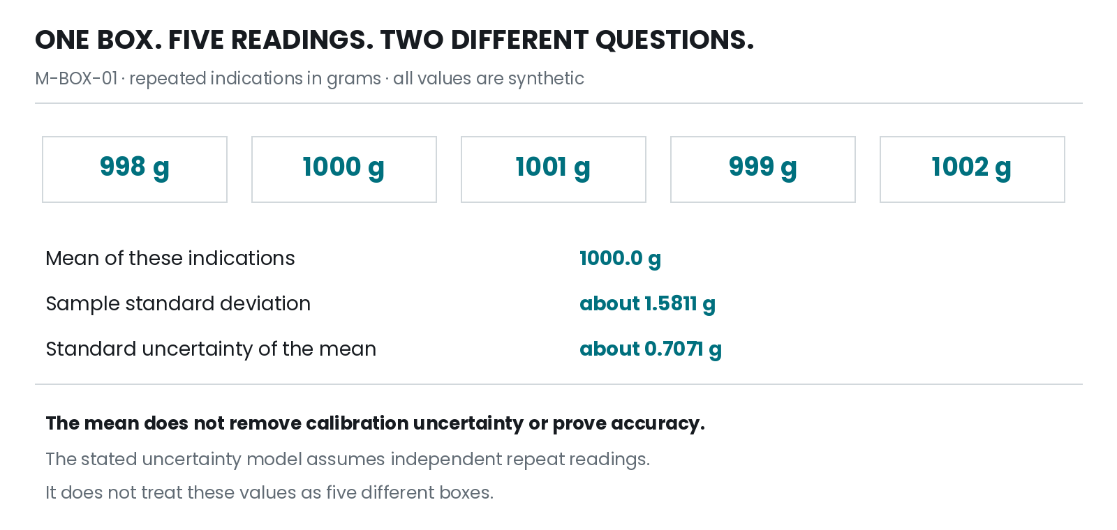
Figure 4.1. Keep the object, procedure, readings and uncertainty model attached to the result. The arithmetic is only one stage of the measurement record.
4.6.4 PLAIN — what is really happening inside#
- The report is applying a measurement model to input estimates and their uncertainty information. That information can come from statistical analysis or from other justified evidence.
- A Type A evaluation uses a statistical analysis of observations. A Type B evaluation uses other available information, such as a calibration report or a specified distribution. These labels describe evaluation methods, not “good” versus “bad” uncertainty. [S32] [S34]
- The model must account for shared effects. When subtracting a tare reading from a gross reading made on the same scale, some offset effects may be shared and may partly cancel. They should not automatically be treated as independent.
- The software should keep enough of the uncertainty budget to explain
the published result. Storing only
plus_minus = 3.3discards the unit, coverage factor, components and assumptions that make the number meaningful.
4.6.5 TECHNICAL — the engineer’s version#
- For a result
y = f(x1, …, xn), first-order uncertainty propagation uses sensitivities of f to the input values, their variances and their covariances. A sensitivity is how much the result changes for a small change in an input. [S31] - For an uncorrelated sum
y = a1*x1 + a2*x2, the combined variance isa1²*u1² + a2²*u2². Taking the square root gives the combined standard uncertainty. This is not the same operation as adding worst-case bounds. - For
net = gross - tare, the general two-input expression is **u_net² = u_gross² + u_tare² - 2*cov(gross, tare)**. Ignoring the covariance assumes something about the relationship between the readings. - In a separate illustrative budget, standard uncertainties of 3 g and 4 g produce 5 g for the difference only when the covariance term is zero. A shared uncertain offset does not satisfy that independence assumption merely because two rows were recorded.
- Strong nonlinearity, awkward distributions, dependent inputs or small-sample effects can require more careful methods than a first-order approximation. This chapter introduces the model; it does not certify every use of its shortcut.
- A machine-readable report could include
estimate,unit,standard_uncertainty,coverage_factor,expanded_uncertainty,method_version,input_observation_idsandassumptions. Include only fields justified by the actual method, rather than filling unknown quantities with invented zeros. - The final quality test is interpretability: can another reader reproduce the arithmetic and distinguish what was observed from what was assumed? A long decimal without that distinction is merely a precise-looking string.
4.6.6 WORDS — remember these#
Standard uncertainty: uncertainty expressed like a standard deviation; technically, measurement uncertainty expressed as a standard deviation under the stated model.
Combined standard uncertainty: the uncertainty after input effects are combined; technically, the standard uncertainty of the result obtained from its input uncertainty model, including relevant dependence.
Expanded uncertainty: a stated multiple of standard uncertainty; technically, U = k × u_combined, accompanied by the coverage factor and justified interpretation.
Covariance: how two quantities vary together; technically, a measure of joint variation that contributes to propagation when input estimates are dependent.
Uncertainty budget: the explanation behind the uncertainty figure; technically, a statement of contributing uncertainty components, their evaluation and their combination in the measurement model.
4.97 Practice and worked answers#
First predict the result#
- An export contains
mass = 1.25without a unit. Can you safely compare it with a record containingmass_g = 1250? - A rectangular label is 25 cm by 40 cm. Calculate its area in square metres and show why a single division by 100 is insufficient.
- Use M-BOX-01 to calculate the mean, sample standard deviation and standard uncertainty of the mean under the stated independent-observation model.
- Two exact decimal inputs are 1.245 and 1.245. Compare half-up rounding to two decimal places before and after addition.
- In the request-timing fixture, what does the 2-second average establish, and what does it leave unknown?
- Combine independent standard uncertainties of 0.70710678 g and 1.5 g, then apply k = 2. Name one assumption that can invalidate a simple interpretation of the resulting interval.
Worked answers#
- No. The first record’s unit and quantity definition are missing. It might be kilograms, grams or something else. A plausible match is not permission to rewrite the source. Obtain the contract or quarantine the ambiguous record.
- The area is 25 × 40 = 1,000 cm². Each square centimetre is 0.0001 m², so the area is 0.1 m². Both length dimensions change scale; therefore the factor is squared.
- The mean is 1,000 g. Squared deviations sum to 10 g², so the sample variance is 10/4 = 2.5 g² and s ≈ 1.58113883 g. Dividing by sqrt(5) gives about 0.70710678 g for the average’s repeatability component, not its complete uncertainty.
- Before addition: 1.25 + 1.25 = 2.50. After addition: 2.490 rounds to 2.49. The procedure must specify where rounding occurs.
- It describes the twelve observed successful completions. It does not establish the mean completion time of all twenty attempts. Under the stated eventual-completion assumptions the latter has a lower bound of 5.2 seconds; without eventual completion a finite all-request mean is not established.
- The combined value is sqrt(2.75) ≈ 1.65831240 g, and the expanded value is approximately 3.31662479 g. Unmodelled shared error, double-counted components or an unjustified distributional assumption can invalidate the intended interpretation.
4.98 Common wrong ideas#
- Wrong: every extra decimal place is extra accuracy. Right: displayed resolution and closeness to the measured quantity are different properties.
- Wrong: a stable instrument must be correct. Right: it can repeat a shared offset consistently.
- Wrong: an average of five readings is the same thing as a typical value for five products. Right: repeated measurements of one object and measurements across different objects answer different questions.
- Wrong: units are decorative labels added at the end. Right: they determine interpretation and can expose invalid calculations before a report is produced.
- Wrong: rounding each input and rounding the final result are interchangeable. Right: the order can change the answer.
- Wrong: missing means zero. Right: replacing absence with zero introduces a substantive assumption.
- Wrong: a low mean among successes proves the service is fast for everyone. Right: excluded timeouts can change the conclusion.
- Wrong: all uncertainty components should be added as independent squares. Right: the model must account for dependence and avoid counting the same effect twice.
- Wrong: k = 2 always guarantees 95% coverage. Right: that interpretation depends on the model and reliability of the uncertainty estimate.
- Wrong: a report is complete once its arithmetic is correct. Right: it also needs the quantity definition, population, method, time boundary and limits of inference.
4.99 Chapter summary in 20 lines#
- Name the quantity intended to be measured before choosing a database field.
- The measurand includes the object and conditions needed to distinguish the intended question.
- Gross mass, tare mass and net mass have different definitions.
- A recorded indication is not automatically a verified physical truth.
- Units travel with values and determine meaningful calculations.
- Converting a squared unit requires squaring its conversion factor.
- Compatible dimensions do not guarantee compatible business meanings.
- Precision concerns agreement among repeated observations under stated conditions.
- Accuracy concerns closeness to the true value and is not itself a numerical percentage in VIM usage.
- A detailed display does not prove a small measurement error.
- The M-BOX-01 readings have mean 1,000 g and sample standard deviation about 1.581 g.
- Under the independent-observation model, their mean’s repeatability uncertainty is about 0.707 g.
- Averaging does not automatically remove shared offsets.
- Rounding needs a scale, a tie rule and a defined place in the calculation.
- Preserve missing observations rather than silently converting them to zero.
- Report denominators and exclusions before generalising an average.
- Uncertainty components need a stated model and a check for dependence.
- The example’s independent components combine to about 1.658 g.
- Multiplying by k = 2 gives about 3.317 g, with coverage interpretation conditional on assumptions.
- A useful measurement report lets the next reader separate observations, calculations and assumptions.